My student days learning fluid dynamics were all about studying complicated equations and various methods of simplifying and manipulating these equations to get some kind of a result. Unfortunately, this left very little to the imagination when it came to getting an intuitive feel for how a fluid would behave in different situations. When I took my first experimental fluid dynamics course, I got to see how one would use different visualization techniques to understand qualitatively the behavior of the flow. These visualizations gave me a way of creatively looking at a flow, and, as an added bonus, they looked stunning. All these experiments and visualizations were being carried out inside a wind tunnel.

Creating Our Computational Wind Tunnel
Wind tunnels are devices used by experimental fluid dynamic researchers to study the effect of an object as it moves through air (or any other fluid). Since the object itself cannot move inside this tunnel, a controlled stream of air, generally produced by a powerful fan, is generated and the object is placed in the path of this stream of air. This produces the same effect as the object moving through stationary air. Such experiments are quite useful in understanding the aerodynamics of an object.
There are different kinds of wind tunnels. The simplest wind tunnel is a hollow pipe, or rectangular box. One end of this tunnel is fitted with a fan, while the other end is open. Such a tunnel is called an open-return wind tunnel. Experimentally, they are not the most efficient or reliable, but would work well if one were to build a computational wind tunnel—which is what we aim to do in this blog post. Here is the basic schematic of the wind tunnel that we will develop:

Our wind tunnel will be a 2D wind tunnel. Fluid will enter the tunnel from the left and leave from the right. The top and bottom are solid walls. I should point out that since this is a computational wind tunnel, we are afforded great flexibility in choosing what kinds of boundaries it can possess. For example, we could make it so that the left, right and bottom walls do not move but the top wall does. We would then have the popular case of flow in a box.
When one starts thinking of computational fluid dynamics, our thoughts invariably jump to the famous Navier–Stokes equations. These equations are the governing equations that dictate the behavior of fluid flow. At this point, it might seem like we are going to use the Navier–Stokes equations to help us build a wind tunnel. But as it turns out, there are other methods to study the behavior of fluid flow without solving the Navier–Stokes equations. One of those methods is called the lattice Boltzmann method (LBM).
If we were to use the Navier–Stokes equations, we would be dealing with a complicated system of partial differential equations (PDEs). To solve these numerically, we would have to employ various techniques to discretize the derivatives. Once the discretization is done, we are left with a massive system of nonlinear algebraic equations that has to be solved. This is computationally exhausting! Using the alternative approach of the LBM, we completely bypass this traditional approach. There are no systems of equations to solve in the LBM. Also, a lot of the operations (which I will describe later) are completely local operations. This makes the LBM a highly parallel method.
In a very simplistic framework, we can think of the LBM as a “bottom-up” approach. In this approach, we perform the simulations in the microscopic, or “lattice,” domain. Imagine you have a physical or macroscopic domain. If we were to zoom in on a single point in this macroscopic domain, there would be a number of particles that are interacting with each other based on some “rule” about their interaction:

For example, if two particles hit each other, how would they react or bounce off each other? These particles follow some discrete rule. Now, if we were to let these particles evolve over time based on these rules (you can see how this is closely related to cellular automata) and take averages, then these averages could be used to describe certain macroscopic quantities. As an example, the HPP model (named after Hardy, Pomeau and de Pazzis) we saw in the previous figure can be used to simulate the diffusion of gases.
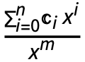
Though this discrete approach sounds enticing (and researchers in the mid-1970s did try out its feasibility), it has a number of drawbacks. One of the major issues was the statistical noise in the final result. However, it is from these principles and attempts to overcome the drawbacks that the LBM emerged. A web search on theoretical aspects of this method will reveal many links to derivations and the final equations. In this blog, rather than focus on the theoretical aspect, I would like to focus on the final underlying mechanism through which the lattice Boltzmann simulations are performed. So I will only touch on the final equations we will need to develop our wind tunnel. First, assume that the density and the velocities are described by the following equations:

… where the fi are called distribution functions and ex, i, ey, i are discrete velocities and have the following values:

The computation of the density and velocities can be done as follows:
✕
ex = {1, 1, 0, -1, -1, -1, 0, 1, 0};
	ey = {0, 1, 1, 1, 0, -1, -1, -1, 0};
	LBMDensityAndVelocity[f_] := Block[{rho, u, v},
	   rho = Total[f, {2}];
	   u = (f.ex)/rho;
	   v = (f.ey)/rho;
	   {rho, u, v}
	   ];
|
These nine discrete velocities are associated with their respective distribution functions fi and can be visualized as follows:

At each (discrete) point in the lattice domain, there will exist nine of these distribution functions. A model that uses these nine discrete velocities and functions fi is called the D2Q9 model. If the distribution functions fi are known, then the velocity field is known. Since the velocity field evolves over space and time, we must expect these distribution functions to also evolve over space and time. The equation governing the spatio-temporal evolution of fi is given by:

The term Ωi is a complicated “collision” term that basically dictates how the various fi interact with each other. Using a number of simplifications and approximations, this equation is reduced to the following:

… where fieq is called the equilibrium distribution function, τ is called the relaxation parameter and δtLBM = 1 is the time step in the lattice Boltzmann domain. This approximation is called the BGK approximation, and the resulting model is called the lattice BGK model. The detailed definitions of these two terms will be provided later. The spatial and temporal evolutions of these functions are done in two steps: (a) the streaming step; and (b) the collision step.
Since δtLBM = 1 and the  are all 1 or 0, the streaming step is given by:

To visualize the streaming step, imagine the discretized domain. On each grid point of this domain are nine of these distribution functions (as shown in the following figure). Note the various colors for each of the grid points. The length of each arrow indicates the magnitude of the respective distribution functions:

Based on the mathematical formulation, each distribution will be streamed in the respective directions as follows:

Note the colors and where they ended up. It would be helpful to just focus on the center point. Before the streaming step, the arrows (which represent the different fi) are all green. After the streaming step, notice where the green arrows land on the surrounding grid points. This, in short, is the streaming step. In Mathematica, this step is done very easily using the built-in functions RotateLeft or RotateRight. Here, we will be using RotateRight:
✕
right = {0, 1};
	left = {0, -1};
	bottom = {1, 0};
	top = {-1, 0};
	none = {0, 0};
	streamDir = {right, top + right, top, top + left, left, bottom + left,
	    bottom, bottom + right, none};
	LBMStream[f_] :=
	  Transpose[
	   MapThread[Flatten[RotateRight[#1, #2]] &, {f, streamDir}]];
|
When one does the streaming, special care has to be taken to address the boundaries of the wind tunnel. When the streaming is done, there are certain fi that become unknown at the edges and corners of the domain. The schematic (shown in the following figure) shows which fi are unknown for their respective edges and corners. The unknowns are represented by dashed arrows:

To understand how the unknown fi are computed, let us consider the top wall of the wind tunnel. For this edge, f6, f7, f8 are unknowns. We let:

 is a two-dimensional unknown vector,
  and fieq are the equilibrium distribution functions and are defined as:

The details of this approach are given in the paper by Ho, Chang, Lin and Lin. This operation (which is actually a highly parallelizable operation) can be done efficiently in Mathematica as:
✕
wts = {1/9, 1/36, 1/9, 1/36, 1/9, 1/36, 1/9, 1/36, 4/9};
	LBMEquilibriumDistributions[rho_, u_, v_] :=
	  Module[{uv, euv, velMag},
	   uv = Transpose[{u, v}];
	   euv = uv.{ex, ey};
	   velMag = Transpose[ConstantArray[Total[uv^2, {2}], 9]];
	   (Transpose[{rho}].{wts})*(1 + 3*euv + (9/2)*euv^2 - (3/2)*velMag)
	   ];
|
Notice that fieq are completely defined by the velocity and density. Substituting this into the equations for velocity and density, we get:

… where UBC, VBC are the velocities specified by the user for the boundary. These resulting equations are linear. There are three unknowns {ρ, Qx, Qy}, and there are three equations. These systems can easily be solved using LinearSolve or Solve. The same procedure can be used for all the edges and corners. Since this is a small 3 × 3 system, we can precompute the expressions for the missing distributions symbolically. So for the top wall, we would have:
✕
Clear[f, feq, rho, ubc, vbc];
	feq = EquilibriumDistributions[{rho}, {ubc}, {vbc}][[1]];
	eqn1 = rho*ubc == Sum[ex[[i]]*f[i], {i, 5}] + Sum[ex[[i]]*(feq[[i]] +
	        wts[[i]]*(ex[[i]]*qx + ey[[i]]*qy)), {i, 6, 8}] + ex[[9]]*f[9];
	eqn2 = rho*vbc == Sum[ey[[i]]*f[i], {i, 5}] + Sum[ey[[i]]*(feq[[i]] +
	        wts[[i]]*(ey[[i]]*qx + ey[[i]]*qy)), {i, 6, 8}] + ey[[9]]*f[9];
	eqn3 = rho == Sum[f[i], {i, 5}] + Sum[(feq[[i]] +
	       wts[[i]]*(ey[[i]]*qx + ey[[i]]*qy)), {i, 6, 8}] + f[9];
	res = FullSimplify[First[Solve[{eqn1, eqn2, eqn3}, {rho, qx, qy}]]]
|
Once {ρ, Qx, Qy} are known, we then substitute the values and obtain the unknowns:
✕
FullSimplify[Table[(feq[[i]] + wts[[i]]*(ey[[i]]*qx
	        + ey[[i]]*qy)), {i, 6, 8}] /. res]
|
When dealing with outflow boundary conditions, we are essentially trying to impose a 0-gradient condition across the boundary, i.e.  . The simplest thing one can do is to use the velocity from one grid behind and use that to compute fi at the boundaries. However, that leads to inaccurate and, in many cases, unstable results.
Consider the right wall as shown in the following figure:

After the streaming step, the distributions f4, f5, f6 are unknown. To impose an outflow condition on the distribution functions fi, we use the following relation:

… where  is the velocity from the previous time step at grid points (j, k), j = 1, 2, …, M and fi,N(t) are the distributions at the previous time step. The scalar term u* must be positive. A good candidate is the normal velocity at the boundary, so for the left and right walls
  , and for the top and bottom walls it would be
  . If u* comes out to be 0, it can be replaced by the characteristic lattice velocity. It is important to note that the unknown distributions change depending on which wall has the outflow condition. For example, if it is the top wall, then f6, f7, f8 are unknown. Details of this approach for outflow treatment can be found in the paper by Yang.
A second approach to imposing outflow condition would be to simply do the following:

This method is much simpler than the first one, and is based on applying a second-order backward difference formula to each of the distribution functions.
Once the streaming is done and boundary conditions are imposed, a “collision” is performed (recall the rule-based approach). This step is basically figuring out how the ensemble-averaged particles are going to interact with each other. This step is a bit complicated, but using the BKG approximation, the collision step can be written as:

… where  are the density and velocities computed after the streaming step and boundary-adjustment step. The term vLBM is the kinematic viscosity in the lattice Boltzmann domain, and τ is the relaxation parameter. This term is quite important and will be discussed in a bit.
This translates to two very simple lines of code in Mathematica:
✕
LBMCollide[f_, u_, v_, rho_, tau_] := Block[{feq},
	   feq = EquilibriumDistributions[rho, u, v];
	   f + (feq - f)/tau
	   ];
|
From a visual standpoint, after the collision, the distribution functions are adjusted based on the previous formula, and we get new distributions:

Notice the change in the lengths of the arrows. That’s it! That is all it takes to run a lattice Boltzmann simulation.
Bringing Simulation to Reality with the Reynolds Number
So how is something like this supposed to simulate the fabled Navier–Stokes equations? To answer that question, we would have to go into a lot of math and multiscale analysis, but in short, the form of feq dictates the macroscopic equations that the LBM simulates. So it is actually possible to simulate a whole bunch of PDEs by using the appropriate equilibrium functions. Once again, I will leave it to the reader to go out into the internet world and get a sample of the remarkable things people simulate using the LBM.
Having seen the basic mechanism of the LBM, the obvious next question is: how do the simulations that are performed in the lattice-based system translate to the physical world? This is done by matching the non-dimensional parameters of the lattice system and the physical system. In our case, it is a single non-dimensional parameter: the Reynolds number. The Reynolds number (Rey) is defined as:

… where Uphy is a characteristic velocity, Lphy is the characteristic length and vphy is the kinematic viscosity in the physical domain. In order to simulate the flow, the user is expected to specify the Reynolds number, the characteristic velocity and the characteristic length. From these three pieces of information, the kinematic viscosity is determined, and subsequently the relaxation parameter τ is determined. Using these pieces of information and the underlying equations associated with the LBM, the internal parameters of the simulation are computed.
The characteristic lattice velocity ULBM must never exceed  (this number is computed to be the speed of sound in the lattice domain). The lattice velocity must remain significantly below this value for it to properly simulate incompressibility. In general, the lattice velocity is taken to be ULBM = 0.1. Similarly, the characteristic lattice length LLBM represents the number of points used in the lattice domain to represent the characteristic length in the physical domain. LLBM would be an integer quantity, and is typically user defined.
Let us look at an example to solidify how to relate the lattice simulation to the physical simulation. Let us assume that Rey = 100, Uphy = 1, Lphy = 1 and the physical dimensions of the wind tunnel are Lw = 15 Lphy, Hw = 5Lphy. For the lattice domain, we assume ULBM = 0.1, LLBM = 10. The lattice wind tunnel dimensions are then LW,LBM = 15 × 10 = 150 and Hw,LBM = 50. The viscosity in the lattice domain is:

This means that the relaxation parameter τ in the BGK model is:

We now have all the quantities we need to run the simulation. If we now let each lattice time step in the simulation be δtLBM = 1, then we need to know what δtphy is. This is done by equating the viscosities and is given by:

Therefore, if we want to run our simulation for t = 100 (time units), then in the lattice domain we would be iterating for  steps.
The Reynolds number is a remarkable non-dimensional parameter. Rather than specify what fluid we are simulating at what velocities and at what dimension, the Reynolds number ties them all together. This means that if we have two systems of vastly different length, velocity scale and fluid medium, the two flows will behave the same as long as the Reynolds number remains the same.
Adding Objects to the Wind Tunnel
Let us now talk about how to introduce objects into the wind tunnel. One approach would be to discretize the objects into a jagged “steps” version of the original object and align it with the grid, then impose a no-slip boundary condition on each one of the step edges and corners:

This is really not a good approach because it distorts the original object; if one needed a good representation of the object, they would have to use an extremely fine grid—making it computationally expensive and wasteful. Furthermore, sharp corners can often induce unwanted behavior in the flow. A second approach would be to immerse the object into the grid. The boundary of the object is discretized and is immersed into the domain:

Discretizing the boundary of a specified object can easily be done using the built-in function BoundaryDiscretizeRegion. We can specify Disk or Circle to generate a set of points that represents the discretized version of the circular object:
✕
bmr = BoundaryDiscretizeRegion[Disk[]];
	pts = MeshCoordinates[bmr];
	Show[bmr, Graphics[Point[pts]], ImageSize -> 250]
|
This method of discretizing the object and placing it inside the grid is called the immersed boundary method (IBM). Once the discretized object is immersed, the effect of that object on the flow needs to be modeled while making sure that the velocity conditions of the boundary are respected. One method of making the flow “feel the presence” of the immersed object is through a method called the direct forcing method. With this approach, the lattice BGK model is modified by adding a forcing term Fi to the evolution equation:

… where  is the corrective force induced on a grid point by the object boundaries. The equation for computing the velocity is now modified as:

The corrective force  is computed as:

… where  are the boundary conditions of the object,
  are the velocities at the object boundaries if the object was not present,
  is an approximation to the delta function and
  are the positions of the boundary points of the object and are generally called Lagrangian boundary points. There are several choices that one can use. We will make use of the following compactly supported function:

This approximation is also called the mollifier kernel and can be defined using the Piecewise function:
✕
Clear[deltaFun];
	deltaFun[r_?NumericQ] :=
	  Piecewise[{{(5 - 3 Abs[r] - Sqrt[1 - 3 (1 - Abs[r])^2])/6,
	     0.5 <= Abs[r] <= 1.5}, {(1 + Sqrt[1 - 3 r^2])/3,
	     Abs[r] <= 0.5}}];
|
✕
Plot[deltaFun[r], {r, -2, 2}, ImageSize -> 300]
|
The 2D function δ(x – X, y – Y) is then given by:

… where dx, dy are scaling parameters. For Lagrangian point (Xi, Yi), a δ function is specified. Here is what the delta function would look like if centered at (1/2,1/2) and scaled by 1:
✕
Plot3D[deltaFun[(x - 1/2)]*deltaFun[(y - 1/2)], {x, -2, 2}, {y, -2,
	  2}]
|
Let’s look at an example to demonstrate this immersed boundary concept, as well as how the function  is constructed and how it is used for approximating a function. Assume that a circle is immersed in a rectangular domain:
✕
Clear[deltaFun];
	deltaFun[r_?NumericQ] :=
	  Piecewise[{{(5 - 3 Abs[r] - Sqrt[1 - 3 (1 - Abs[r])^2])/6,
	     0.5 <= Abs[r] <= 1.5}, {(1 + Sqrt[1 - 3 r^2])/3,
	     Abs[r] <= 0.5}}];
|
✕
ng = N[Range[-2, 2, 4/30]];
	dx = dy = ng[[2]] - ng[[1]];
	grid = Flatten[Outer[List, ng, ng], 1];
	n = 30;
	bpts = N[CirclePoints[n]];
	Graphics[{{Red, PointSize[0.03], Point[bpts]}, {Blue, Point[grid]}},
	 ImageSize -> 300]
|
Each Lagrangian boundary point (in blue) influences the grid points (various intersections of the vertical and horizontal lines) within a certain radius, as shown in the following figure:

To get the grid points that are influenced by each of the Lagrangian points, we make use of the Nearest function:
✕
dr = 1.5 Sqrt[dx^2 + dy^2];
	nf = Nearest[grid -> Automatic];
	influenceGridPtsIndex = nf[bpts, {Infinity, dr}];
|
The function δ(x – X(s), y – Y(s)) for discrete points essentially becomes a matrix:
✕
gp = grid[[#]] & /@ influenceGridPtsIndex;
	dd = MapThread[Transpose[#1] - #2 &, {gp, bpts}];
	dval = Table[
	   Map[deltaFun[#/dx] &, di[[1]]]*Map[deltaFun[#/dy] &, di[[2]]], {di,
	     dd}];
	t = Flatten[
	   MapThread[
	    Thread[Thread[{#1, #2}] -> #3] &, {Range[n],
	     influenceGridPtsIndex, dval}]];
	dMat = SparseArray[t, {n, Length[grid]}]
|
This matrix can now be used to compute the values at the Lagrangian points. For example, let us assume that the underlying grid has values on it defined by h(x, y) = Sin(x + y), then the values at the Lagrangian points are computed as:

... where D is the discretization of δ and h(xj, yj) are the function values to be computed at (xj, yj):
✕
bptVal = dMat.Sin[Total[grid, {2}]];
|
We can compare the computed interpolated value to the actual values:
✕
ListLinePlot[{bptVal, Sin[Total[bpts, {2}]]}, ImageSize -> 300,
	 PlotStyle -> {Red, Black}, PlotLegends -> {"Computed", "Actual"}]
|
Similarly, the function values at the grid can be computed using the function values at the Lagrangian points as:
✕
wts = IdentityMatrix[n];
	wts[[1, 1]] = wts[[-1, -1]] = 0.5;
	wts *= (Norm[bpts[[2]] - bpts[[1]]])/(dx*dy);
	gridVal = Sin[Total[bpts, {2}]].wts.dMat;
	hfun = Interpolation[Transpose[{grid, gridVal}]];
	Plot3D[hfun[x, y], {x, -2, 2}, {y, -2, 2}, PlotRange -> All]
|
As you can see, since the δ functions have compact support, only grid points that lie in their radius of influence get interpolated values. All grid points that are not in their support radius are 0.
So, to remind the readers, one single step in the lattice Boltzmann simulation consists of the following steps:
- Perform the streaming step.
- Adjust distribution functions at the boundaries.
- Perform the collision step.
- Compute the velocities
 .
.
- Compute the velocities
 at the Lagrangian boundary points of the objects.
- For each boundary point of the object, compute the corrective force needed to enforce the boundary conditions at that point.
- Compute the corrective forces
 at the lattice grid points using the forces obtained in step 6.
- Perform the streaming and collision steps, taking the forces into account.
- Calculate density and velocities.
This concludes all the necessary ingredients needed to run a wind tunnel simulation using the LBM in 2D.
Examples
To make this wind tunnel easy to use, I have put all these functions into a package called WindTunnel2DLBM. It contains a number of features and allows for easy setup of the problem by a user. I would recommend the interested user go through the package documentation for details. The focus here will be on the various examples and the flexibility our computational wind tunnel setup offers.
The first example is the flow in the wind tunnel. This is perhaps the simplest case. A schematic of the domain and its associated boundary conditions are shown here:

In this case, there is only one length scale to the problem: the height of the wind tunnel. Therefore, that becomes our characteristic length scale. The characteristic velocity in this case is the maximum velocity coming from the inlet, which is set to 1. All that remains is to specify the Reynolds number at which the simulation is to be carried out. This is user defined as well. Let us take the length of the wind tunnel to be 6 units going from (0,6), and the height to be 2 units going from (-1,1). We now set up the simulation:
✕
<< WindTunnel2DLBM`;
|
✕
Rey = 200;
	charLen = 1;
	charVel = 1;
	ic  = Function[{x, y}, {0, 0}];
	state = WindTunnelInitialize[{Rey, charLen, charVel},
	  ic, {x, 0, 6}, {y, -1, 1}, t]
|
Notice that we did not provide any boundary condition information here. That is because the wind tunnel defaults to the flow in a channel case, and therefore all the boundary conditions are automatically imposed. All we have to specify are the characteristic information and the dimensions of the wind tunnel.
The simulation is performed using a fixed time step. The time step is internally computed and can be accessed from the following property:
✕
state["TimeStep"]
|
Let us now run the simulation for a period of 5 time units:
✕
WindTunnelIterate[state, 5];
	state
|
We can query the data at the final step of the simulation:
✕
{usol, vsol} = {"U", "V"} /. state[state["CurrentTime"]];
|
The solution can be visualized in a variety of ways. For 2D simulation, a streamline plot can reveal some useful information. Let us visualize the streamline plot:
✕
StreamPlot[{usol[x, y], vsol[x, y]}, {x, 0, 6}, {y, -1, 1},
	 AspectRatio -> Automatic, ImageSize -> 400, PlotRangePadding -> None]
|
Notice that the streamlines are not completely parallel (there is a bit of deviation). To see why, let us look at the profiles of the u component of the velocity field at various x locations:
✕
Plot[Evaluate[{usol[#, y] & /@ Range[0, 6, 2]}], {y, -1, 1},
	 ImageSize -> 300, PlotLegends -> Range[0, 6, 2],
	 PlotStyle -> {Black, Red, Blue, Green}]
|
This indicates that the velocities have a spatial dependence. For this particular problem, we should expect the flow to reach steady state, i.e. the flow should not vary with time. Let us run the simulation for an additional 20 time units and see the velocity profile:
✕
WindTunnelIterate[state, 20];
	{usol, vsol} = {"U", "V"} /. state[state["CurrentTime"]];
	Plot[Evaluate[{usol[#, y] & /@ Range[0, 6, 2]}], {y, -1, 1},
	 ImageSize -> 300, PlotLegends -> Range[0, 6, 2],
	 PlotStyle -> {Black, Red, Blue, Green}]
|
We see that the velocity profiles at the various x locations are almost the same as each other. This gives us an indication that the flow is indeed reaching steady state.
The Flow-in-a-Box Problem
Let us now look at the classic flow-in-a-box problem. Here’s the schematic of the domain and the boundary condition information:

The top wall moves with a horizontal velocity of 1 (length units/time units), while all the others are stationary, no-slip walls. The circles inside the box denote the kind of fluid behavior that might be expected. As the top wall moves, the wall drags the fluid below it, causing the fluid to rotate—that is the big circle in the schematic, and it represents a vortex. If there is sufficient strength in the main vortex, then we can expect it to start causing smaller, secondary vortices to form. Our hypothesis is that the strength of the vortex should be related to the Reynolds number. Let us see what happens by running the simulation at Reynolds number 100:
✕
state = WindTunnelInitialize[{100, 1, 1},
	   Function[{x, y}, {0, 0}], {x, 0, 1}, {y, 0, 1}, t,
	   "CharacteristicLatticePoints" -> 60,
	   "TunnelBoundaryConditions" -> {"Left" -> "NoSlip",
	     "Right" -> "NoSlip", "Bottom" -> "NoSlip",
	     "Top" -> Function[{x, y, t}, {1, 0}]}];
|
We now iterate for 50 time units:
✕
WindTunnelIterate[state, 50];
|
Visualizing the result shows us that there is a primary vortex that forms near the middle, while a smaller, secondary vortex forms at the bottom right of the box:
✕
{usol, vsol} = {"U", "V"} /. state[state["CurrentTime"]];
	StreamPlot[{usol[x, y], vsol[x, y]}, {x, 0, 1}, {y, 0, 1},
	 AspectRatio -> Automatic, StreamPoints -> Fine,
	 PlotRangePadding -> None, ImageSize -> 300]
|
If the Reynolds number is ramped up, then these secondary vortices become stronger and larger, and additional vortices start developing in the corners. Let us look at the case when the Reynolds number is 1,000:
✕
state = WindTunnelInitialize[{1000, 1, 1},
	   Function[{x, y}, {0, 0}], {x, 0, 1}, {y, 0, 1}, t,
	   "CharacteristicLatticePoints" -> 60,
	   "TunnelBoundaryConditions" -> {"Left" -> "NoSlip",
	     "Right" -> "NoSlip", "Bottom" -> "NoSlip",
	     "Top" -> Function[{x, y, t}, {1, 0}]}];
|
We will again iterate for 50 time units:
✕
WindTunnelIterate[state, 50];
|
Let us visualize the result:
✕
{usol, vsol} = {"U", "V"} /. state[state["CurrentTime"]];
	StreamPlot[{usol[x, y], vsol[x, y]}, {x, 0, 1}, {y, 0, 1},
	 AspectRatio -> Automatic, StreamPoints -> Fine,
	 PlotRangePadding -> None, ImageSize -> 300]
|
Notice that the primary vortex has moved closer to the center; from the looks of it, it’s strong enough to be able to form secondary vortices at the bottom left and bottom right of the domain.
Let us now see what happens if we do the simulation on a “tall” box rather than a square one. The boundary conditions remain the same, but the domain changes in the y direction:
✕
state = WindTunnelInitialize[{1000, 1, 1},
	   Function[{x, y}, {0, 0}], {x, 0, 1}, {y, 0, 2}, t,
	   "CharacteristicLatticePoints" -> 60,
	   "TunnelBoundaryConditions" -> {"Left" -> "NoSlip",
	     "Right" -> "NoSlip", "Bottom" -> "NoSlip",
	     "Top" -> Function[{x, y, t}, {1, 0}]}];
|
Run the simulation and use ProgressIndicator to track the progress. This simulation will take a few minutes:
✕
ProgressIndicator[Dynamic[state["CurrentTime"]], {0, 50}]
	AbsoluteTiming[WindTunnelIterate[state, 50]]
|
Visualize the streamlines:
✕
{usol, vsol} = {"U", "V"} /. state[state["CurrentTime"]];
	StreamPlot[{usol[x, y], vsol[x, y]}, {x, 0, 1}, {y, 0, 2},
	 AspectRatio -> Automatic, StreamPoints -> Fine,
	 PlotRangePadding -> None, ImageSize -> Medium]
|
In the tall-box scenario, a primary vortex is developed near the top wall, and that vortex in turn creates another vortex below it. If that second vortex is strong enough, it will create vortices at the bottom corners of the box.
We can already see the flexibility our wind tunnel is providing us. Let us now put an object inside the wind tunnel and observe the behavior of the flow. For this example, use a circular object:

This is the same as flow in a channel (our first example), but with an object placed in the channel. Notice now that there are are two length scales d and H. The choice of the characteristic length, though arbitrary, must tie back to some aspect of the physics of the flow. In this example, if the size of the object was to be increased or decreased, then the flow pattern behind it would be expected to change. Therefore, the natural choice is to use d as the characteristic length.
Let us place the cylinder at (3,0) in the domain. Let the size of the cylinder be 1 length unit. Therefore, the characteristic scale will be 1. Let the domain size be (0, 15) × (–2, 2). The object is specified as a ParametricRegion:
✕
Remove[state];
	state = WindTunnelInitialize[{200, 1, 1},
	  Function[{x, y}, {0, 0}], {x, 0, 15}, {y, -2, 2}, t,
	  "CharacteristicLatticePoints" -> 15,
	  "ObjectsInTunnel" -> {ParametricRegion[{3 + Cos[s]/2,
	      Sin[s]/2}, {{s, 0, 2 Pi}}]}]
|
It is a good idea to visualize the tunnel before starting the simulation, to make sure the object is in the correct position:
✕
ListLinePlot[state["ObjectsInTunnel"],
	 PlotRange -> {{0, 14}, {-2, 2}}, AspectRatio -> Automatic,
	 Axes -> False, Frame -> True, ImageSize -> Medium,
	 PlotLabel ->
	  StringForm["GridPoints: ``", Reverse@state["GridPoints"]]]
|
Let us simulate the flow for 10 time units:
✕
WindTunnelIterate[state, 10];
	{usol, vsol} = {"U", "V"} /. state[state["CurrentTime"]];

	Rasterize@
	 Show[LineIntegralConvolutionPlot[{{usol[x, y], vsol[x, y]}, {"noise",
	      300, 400}}, {x, 0, 15}, {y, -2, 2}, AspectRatio -> Automatic,
	   ImageSize -> Medium, PlotRangePadding -> None,
	   LineIntegralConvolutionScale -> 2, ColorFunction -> "RoseColors"],
	  ListLinePlot[state["ObjectsInTunnel"],
	   PlotStyle -> {{Thickness[0.005], Black}}]]
|
There are two things to notice here: the symmetric pair of vortices behind the cylinder and the flow inside the cylinder. A close-up reveals that there is some flow pattern inside the cylinder as well:
✕
Show[StreamPlot[{usol[x, y], vsol[x, y]}, {x, 2.4, 3.6}, {y, -1/2,
	   1/2}, AspectRatio -> Automatic, ImageSize -> Medium,
	  PlotRangePadding -> None],
	 ListLinePlot[state["ObjectsInTunnel"],
	  PlotStyle -> {{Thickness[0.01], Blue}}]]
|
This behavior is because we are making use of the IBM. As mentioned earlier, the IBM computes a set of forces to be applied on the grid points such that the velocity at the surface representing the surface is 0. It does not specify what needs to happen inside the cylinder. Therefore, being an incompressible flow, there exists a flow pattern inside the cylinder as well. The important thing is that the velocities at the boundaries of the object are 0 (no-slip).
Let us now continue to iterate for 30 time units and see what happens to the pattern behind the cylinder. Sometimes, it can be helpful to look at another variable called vorticity to get a better understanding of what is happening:
✕
WindTunnelIterate[state, 30];
	{usol, vsol} = {"U", "V"} /. state[state["CurrentTime"]];
|
Set up the color scheme for the contours:
✕
cc = N@Range[-3, 3, 4/100];
	cc = DeleteCases[cc, x_ /; -0.4 <= x <= 0.4];
	cname = "VisibleSpectrum";
	cdata = ColorData[cname];
	crange = ColorData[cname, "Range"];
	cMinMax = {Min[cc], Max[cc]};
	colors = cdata[Rescale[#, cMinMax, crange]] & /@ cc;
|
Visualize the vorticity:
✕
Remove[vort];
	vort = D[usol[x, y], y] - D[vsol[x, y], x];
	Rasterize@Show[ContourPlot[vort, {x, 0, 15},
	   {y, -2, 2}, AspectRatio -> Automatic, ImageSize -> 500,
	   Contours -> cc, ContourShading -> None, ContourStyle -> colors,
	   PlotRange -> {{0, 15}, {-2, 2}, All}],
	  Graphics[Polygon[state["ObjectsInTunnel"]]]]
|
We now notice that the symmetric pattern has been destroyed and is replaced by this “wavy” behavior; the vorticity clearly shows the wavy behavior. What we notice here is called an instability in the wake of the cylinder. This instability continues to amplify, and eventually vortices start forming behind the cylinder. This phenomenon is called “vortex shedding.” There is a shear layer generated at the surface of the cylinder that gets carried downstream.
This vortex shedding is also dependent on the Reynolds number. For small enough numbers, we don’t get any shedding. However, at around 100–150, the shedding is observed. To properly observe this phenomena, it would be good to see the time evolution of this flow. As a first step, set up the problem by defining the characteristic terms and the objects in the tunnel:
✕
state = WindTunnelInitialize[{200, 1, 1},
	   Function[{x, y}, {0, 0}], {x, 0, 15}, {y, -2, 2}, t,
	   "CharacteristicLatticePoints" -> 15,
	   "ObjectsInTunnel" -> {ParametricRegion[{3 + Cos[s]/2,
	       Sin[s]/2}, {{s, 0, 2 Pi}}]}];
|
To produce a time evolution of the vorticity, we will extract the solution at each time unit and generate a series of plots:
✕
cc = N@Range[-5, 5, 10/200];
	cc = DeleteCases[cc, x_ /; -0.5 <= x <= 0.5];
	cname = "VisibleSpectrum";
	cdata = ColorData[cname];
	crange = ColorData[cname, "Range"];
	cMinMax = {Min[cc], Max[cc]};
	colors = cdata[Rescale[#, cMinMax, crange]] & /@ cc;

	res = Table[
	   WindTunnelIterate[state, t];
	   {usol, vsol} = {"U", "V"} /. state[state["CurrentTime"]];
	   vort = D[usol[x, y], y] - D[vsol[x, y], x];
	   plot =
	    Show[ContourPlot[vort, {x, 0, 15}, {y, -2, 2},
	      AspectRatio -> Automatic, ImageSize -> Medium, Contours -> cc,
	      ContourShading -> None, ContourStyle -> colors,
	      PlotRange -> {{0, 15}, {-2, 2}, All}],
	     Graphics[Point /@ state["ObjectsInTunnel"]]];
	   Rasterize[plot]
	   , {t, 0, 50, 1}];
|
Running the simulation clearly shows two vortices forming in the back of the cylinder with the shear layer slowly getting perturbed, which then increases in amplitude before finally breaking into a vortex shedding:
✕
ListAnimate[res, DefaultDuration -> 10, AnimationRunning -> False]
|
Observing Disturbances Caused by a Moving Object
For our next example, we will exploit the immersed boundary treatment and “immerse” a circular tank inside our wind tunnel. The boundary of the tank will have 0-velocities. Inside this tank, we will immerse an elliptical object. This object is placed near the tank wall and follows the tank boundary in a circular path. The flexibility of the lattice Boltzmann method with immersed boundary allows us great flexibility with moving objects. The objective is to study what kind of disturbances develop when this object moves through a still fluid.
Set up the problem by defining the characteristic terms. In this case, the simulation will be performed at a Reynolds number of 400. The characteristic length and velocity are specified as unity. There are two objects in the tunnel. The first object is the large circular tank that is held stationary; the second is the elliptical object that will be moving inside this tank:
✕
Remove[state];
	state = WindTunnelInitialize[{400, 1, 1},
	  Function[{x, y}, {0, 0}], {x, -2.2, 2.2}, {y, -2.2, 2.2}, t,
	  "CharacteristicLatticePoints" -> 25,
	  "TunnelBoundaryConditions" -> {"Left" -> "NoSlip",
	    "Right" -> "NoSlip", "Top" -> "NoSlip", "Bottom" -> "NoSlip"},
	  "ObjectsInTunnel" -> {{ParametricRegion[{1.3 + 0.2*Sin[s],
	       0.5*Cos[s]}, {{s, 0, 2 Pi}}], Function[{xb, yb, t}, {-yb, xb}]},
	    {ParametricRegion[{2*Sin[s], 2*Cos[s]}, {{s, 0, 2 Pi}}]}}]
|
As always, it is a good idea to check the geometry of the underlying problem. We can do that by simply extracting the discretized object when doing the initialization; we can see that everything is where it is supposed to be:
✕
Graphics[Map[Line, state["ObjectsInTunnel"]], Frame -> True,
	 ImageSize -> Small]
|
As we did before, we will be looking at the vorticity contours of the flow. Let us first define the color scheme and the levels of contours that will be plotted:
✕
cc = N@Range[-7, 7, 14/100];
	cc = DeleteCases[cc, x_ /; -0.1 <= x <= 0.1];
	cname = "VisibleSpectrum";
	cdata = ColorData[cname];
	crange = ColorData[cname, "Range"];
	cMinMax = {Min[cc], Max[cc]};
	colors = cdata[Rescale[#, cMinMax, crange]] & /@ cc;
|
The simulation is now run for 60 time units:
✕
oreg = RegionPlot[x^2 + y^2 >= 2^2, {x, -2.2, 2.2}, {y, -2.2, 2.2},
	   PlotStyle -> Black];
	AbsoluteTiming[res = Table[
	    WindTunnelIterate[state, tt];
	    {usol, vsol} = {"U", "V"} /. state[state["CurrentTime"]];
	    vort = D[usol[x, y], y] - D[vsol[x, y], x];
	    Rasterize@
	     Show[ContourPlot[vort, {x, -2, 2}, {y, -2, 2},
	       AspectRatio -> Automatic, ImageSize -> 300, Contours -> cc,
	       ContourShading -> None, ContourStyle -> colors,
	       PlotRange -> {{-2, 2}, {-2, 2}, All}],
	      Graphics[Polygon[First[state["ObjectsInTunnel"]]]], oreg], {tt,
	     0, 60, 1/2}];]
|
Running the time evolution of the fluid disturbance shows that a very beautiful geometric pattern is formed within the tank initially before settling down to a more uniform circular disturbance:
✕
ListAnimate[res, DefaultDuration -> 10, AnimationRunning -> False,
	 ImageSize -> Automatic]
|
Flow in a Pipe with Bends and Obstacles
For the sake of curiosity (and fun), what kind of flow pattern would we expect for the following geometry?

Fluid enters the pipe from the right end, moves up the pipe and then gets discharged from the left end. What would be the effect of that stopper at the right end? How will it impact the discharge?
This is surprisingly easy to figure out with our current setup. Again, we just immerse our pipe and the obstacle within it into our wind tunnel. The left, right and top boundaries of the wind tunnel are given a 0-velocity condition. The bottom boundary is given an outflow condition from –1 ≤ x ≤ –0.7, a 0-velocity condition from –0.7 ≤ x ≤ 0.7 and a parabolic velocity profile from 0.7 ≤ x ≤ 1:
✕
Remove[state];
	inletVel = Fit[{{7/10, 0}, {17/20, 1}, {1, 0}}, {1, x, x^2}, x];
	state = WindTunnelInitialize[{500, 0.3, 1},
	  Function[{x, y}, {0, 0}], {x, -1.1, 1.1}, {y, 0, 1.1}, t,
	  "CharacteristicLatticePoints" -> 20,
	  "TunnelBoundaryConditions" -> {"Left" -> "NoSlip",
	    "Right" -> "NoSlip", "Top" -> "NoSlip",
	    "Bottom" ->
	     Function @@
	      List[{x, y, t},
	       If @@ List[0.7 <= x <= 1., {0, inletVel},
	         If[-1 <= x <= -0.7, "Outflow", {0, 0}]]]},
	  "ObjectsInTunnel" -> {ImplicitRegion[
	     0.7 <= (x^4 + y^4)^(1/4) <= 1, {{x, -1, 1}, {y, -0.2, 1}}],
	    ParametricRegion[{0.22 + t, t - 0.2}, {{t, 0.55, 0.7}}]}]
|
Let us run it for 40 time units:
✕
ProgressIndicator[Dynamic[state["CurrentTime"]], {0, 40}]
	AbsoluteTiming[WindTunnelIterate[state, 40]]
|
Let us plot the vorticity:
✕
{usol, vsol} = {"U", "V"} /. state[state["CurrentTime"]];
	vort = D[usol[x, y], y] - D[vsol[x, y], x];
	cc = N@Range[-20, 20, 40/50];
	cc = DeleteCases[cc, x_ /; -0.1 <= x <= 0.1];
	cname = "VisibleSpectrum";
	cdata = ColorData[cname];
	crange = ColorData[cname, "Range"];
	cMinMax = {Min[cc], Max[cc]};
	colors = cdata[Rescale[#, cMinMax, crange]] & /@ cc;
	Rasterize@
	 Show[ContourPlot[vort, {x, -1, 1}, {y, 0, 1},
	   AspectRatio -> Automatic, ImageSize -> Medium, Contours -> cc,
	   ContourShading -> None, ContourStyle -> colors,
	   PlotRange -> {{-1, 1}, {0, 1}, All},
	   RegionFunction -> Function[{x, y}, 0.7 <= (x^4 + y^4)^(1/4) <= 1]]
	  , Graphics[Point /@ state["ObjectsInTunnel"]]]
|
We see that the obstacle/stopper introduces a vortex shedding, which travels down the pipe. Let us look at the velocities at y = 0:
✕
Plot[vsol[x, 0], {x, -1, 1}, PlotRange -> {{-1, 1}, {-1, 1}},
	 ImageSize -> Medium]
|
If we compare the velocity profile between the outlet (at the left) and inlet (at the right), we see that the outlet velocity is almost half of the inlet. This gives us compelling evidence that the stopper has caused a reduction in fluid discharge from the left end of the pipe, which is to be expected.
Simulating the Flow over an Airfoil
As a final example, let us look at the flow around an airfoil. An airfoil basically represents the cross-section of an airplane wing, and is the fundamental thing that actually allows an airplane to lift off the ground. There are many types of airfoils, but we will focus on a simple one where the airfoil is described by the parametric equation  The parameter a controls how thick the airfoil should be, and the parameter b controls the curvature of the airfoil:
✕
Clear[mat, a, b, t, AOA];
	Manipulate[
	 mat = {{Cos[AOA Degree], -Sin[AOA Degree]}, {Sin[AOA Degree],
	    Cos[AOA Degree]}};
	 ParametricPlot[
	  mat.{t^2, 0.2 (t - t^3 + (t^2 - t^4)/b)/a}, {t, -1, 1},
	  AspectRatio -> Automatic, ImageSize -> Medium,
	  PlotRange -> {{0, 1}, {-0.2, 0.5}}], {{a, 1}, 0.1, 10}, {{b, 0.9},
	  0.3, 10}, {{AOA, 0, "Angle of Attack"}, -20, 20}]
|
In order for the aircraft to get “lift,” i.e. be able to get off the ground, the top surface of the airfoil should have a pressure distribution that is lower than the bottom surface. This pressure difference causes the wing to lift upward (along with anything attached to it). This pressure difference is achieved by having wind blow over its surface at significantly high speeds. A second consideration is that the wing generally needs to be tilted or have an “angle of attack” to it. By doing this, we ensure greater lift. We will also give the airfoil a –10° angle of attack. The simulation will be run for a Reynolds number of 1,000. Now, I should point out that a Reynolds number of 1,000 is a rather small value. A typical Reynolds number for small aircraft is around 1 million. A full-scale simulation is just not possible on a laptop because of the large grid size. However, even at 1,000, we should be able to get a good understanding of the underlying dynamics. For this example, a uniform flow fill comes in from the left. The top and bottom tunnel boundaries are set to be periodic, and the right boundary is set to an outflow. The characteristic length here will be the thickness of the airfoil:
✕
state = WindTunnelInitialize[{1000, 0.2, 1},
	  Function[{x, y}, {0, 0}], {x, -2, 6}, {y, -1., 1.}, t,
	  "CharacteristicLatticePoints" -> 20,
	  "CharacteristicLatticeVelocity" -> 0.05,
	  "TunnelBoundaryConditions" -> {"Left" ->
	     Function[{x, y, t}, {1, 0}], "Right" -> "Outflow",
	    "Top" -> "Periodic"},
	  "ObjectsInTunnel" -> {ParametricRegion[{{Cos[-10 Degree], -Sin[-10 \
	Degree]}, {Sin[-10 Degree], Cos[-10 Degree]}}.{t^2,
	       0.2 (t - t^3 + (t^2 - t^4)/0.9)/1}, {{t, -1, 1}}]}]
|
Before starting the simulation, extract the discretized object and check that it is in the appropriate location within the wind tunnel:
✕
ListLinePlot[state["ObjectsInTunnel"],
	 PlotRange -> Evaluate[state["Ranges"]], AspectRatio -> Automatic,
	 Axes -> False, Frame -> True, ImageSize -> 400,
	 PlotLabel ->
	  StringForm["GridPoints: ``", Reverse@state["GridPoints"]]]
|
Notice the large number of grid points. This is because we are allowing 20 lattice points to resolve the thin airfoil. We now run the simulation for 10 time units. This simulation takes a bit of time to finish 10 time units’ worth of simulation because: (a) the resolution (i.e. the number of grid points needed for running this simulation) is quite large (800×200); and (b) to complete the simulation, 20,000 iterations must be performed:
✕
10/state["TimeStep"]
|
Start the iteration process:
✕
AbsoluteTiming[WindTunnelIterate[state, 10]]
|
Let us first look at the vorticity plot:
✕
{usol, vsol} = {"U", "V"} /. state[state["CurrentTime"]];
	vort = D[usol[x, y], y] - D[vsol[x, y], x];
	cc = N@Range[-15, 15, 30/60];
	cc = DeleteCases[cc, x_ /; -0.1 <= x <= 0.1];
	cname = "VisibleSpectrum";
	cdata = ColorData[cname];
	crange = ColorData[cname, "Range"];
	cMinMax = {Min[cc], Max[cc]};
	colors = cdata[Rescale[#, cMinMax, crange]] & /@ cc;
	Show[ContourPlot[vort, {x, -0.5, 5}, {y, -1, 1},
	  AspectRatio -> Automatic, ImageSize -> 500, Contours -> cc,
	  ContourShading -> None, ContourStyle -> colors,
	  PlotRange -> {{-0.5, 5}, {-1, 0.5}, All}]
	 , Graphics[{FaceForm[White], EdgeForm[Black],
	   Polygon[state["ObjectsInTunnel"][[1]]]}]]
|
Just as in the case of the bluff body, we are seeing vortex shedding. For the case of the airfoil, this is not really a desirable property. We ideally want the flow to hug the surface. When the flow separates (as you see on the top surface of the airfoil), the pressure drop is not achieved properly and the airfoil will be unable to generate lift.
Let us now look at the pressure. Rather than plotting the pressure, we will plot a non-dimensional parameter called the pressure coefficient, defined by Cp = 2(p – p∞)/(ρLBM U2LBM), where p∞ is the pressure far upstream. We are interested in looking at the pressure at the object’s surface:
✕
PressureCoefficient[x_?NumericQ,
	  y_?NumericQ] := (psol[x, y] - psol[-2, 0])/(0.5*
	    state["InternalVelocity"]^2)
|
✕
							objs = state["ObjectsInTunnel"][[1]];
psol = "P" /. state[state["CurrentTime"]];
pp = Apply[psol, objs, 1];
	pp = (pp - psol[-2, 0])/(0.5*state["InternalVelocity"]^2);
	ListPlot[Transpose[{objs[[All, 1]], pp}], PlotRange -> All,
	 Axes -> False, Frame -> True,
	 FrameLabel -> {"x \[Rule]", "\!\(\*SubscriptBox[\(C\), \(p\)]\)"},
	 FrameStyle -> Directive[Black, 14], ImageSize -> Medium]
|
You will notice that there are two lines here. The lower line represents the pressure on the top surface, while the top line represents the pressure on the bottom surface. It is clear that despite some separation from the airfoil, we are getting some pressure differences. We can also plot the pressure contours and visualize them near the airfoil:
✕
Show[Quiet@
	  ContourPlot[
	   PressureCoefficient[x, y], {x, -0.5, 1.5}, {y, -0.4, 0.4},
	   AspectRatio -> Automatic, PlotRangePadding -> None,
	   ColorFunction -> "TemperatureMap", Contours -> 40,
	   PlotLegends -> Automatic, PlotRange -> All, ImageSize -> Medium],
	 Graphics[{FaceForm[White], EdgeForm[Black],
	   Polygon[state["ObjectsInTunnel"][[1]]]}]]
|
If you look carefully at the color scheme, you will indeed see that the top-surface pressure is less than the bottom surface. So perhaps there is hope with this airfoil. The fluid-dynamic property that we have just explored is called the Bernoulli principle, which has applications in aviation (as we have seen here) and in fields such as automotive engineering.
This is just the start—there are many more examples you can try out! What we have discussed here is a good place to begin exploring this alternative approach to studying fluid dynamics problems and their implementation in Mathematica. The LBM combined with the IBM is a good tool for anyone interested in studying and analyzing fluid flows. With the help of Mathematica’s built-in functions, putting together the numerical wind tunnel is quite straightforward. The WindTunnel2DLBM package has helped me explore many fascinating concepts in the field of fluid dynamics (and make stunning visualizations). I hope you too will get inspired and dive into the exploration of fluid-flow phenomena.


 One step might surprise you.


 :
:


 and we get:

 as
as 


 such that
  are undetermined coefficients.


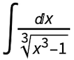 was reduced to
 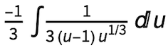 with the substitution u = 1 – x3, while the integral
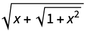
 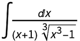 was reduced to
 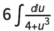 with the substitution s =
  .
. . We can make this substitution with GroebnerBasis as follows:


 and Swissmint for this incredible honour and privilege.


![Clear[f, feq, rho, ubc, vbc];](/data/uploads/2019/11/pm1021img32.png "Clear[f, feq, rho, ubc, vbc];")


![Clear[deltaFun];](/data/uploads/2019/10/pm1021img86.png "Clear[deltaFun];")


![Remove[state];](/data/uploads/2019/10/pm1021img133.png "Remove[state];")


![Remove[state];](/data/uploads/2019/10/pm1021img139.png "Remove[state];")


![Remove[state];](/data/uploads/2019/10/pm1021img143.png "Remove[state];")


![Remove[state];](/data/uploads/2019/10/pm1021img151.png "Remove[state];")


![Clear[deltaFun];](/data/uploads/2019/10/pm1021img161.png "Clear")


