
Most people (including myself) are drawn to Julia by its lofty goals. Speed of C, statistical packages of R, and ease of Python?—it sounds two good to be true. However, I haven't seen anyone who has looked into it say the developers behind the language aren't on track to accomplish these goals.
Having only been around since 2012, Julia's greatest disadvantage is a lack of community support. If you have an obscure Julia question and you google it, you probably won't find the answer, whereas with Python or R or Java you would. This also means less package support. The packages for linear algebra, plotting, and other stuff are there, but if you want to do computer vision or nlp, you'd be among the few.
However, it is definitely worth looking into. I'm not quite a pro, but I'm getting to the point where if I code something in Python, I can easily transfer it to Julia. Then sometimes I test the speed for fun. Julia always wins.
Recently, I wrote an article about linear algebra, with accompanying code in Python. Below is basically the same article, with the code in Julia. If you need help with the basic syntax, I also wrote a basic syntax guide, kind of a compressed version of the documentation. I included the concept descriptions, but they're no different from my original article. The point of this is just to show how easy it is to do linear algebra in Julia.
Here is the iPython notebook on my github. (You can write Julia code in iPython...it's awesome).
The Basics
matrix – a rectangular array of values
vector – one dimensional matrix
identity matrix I – a diagonal matrix is an n x n matrix with one’s on the diagonal from the top left to the bottom right.
i.e.
[[ 1., 0., 0.],
[ 0., 1., 0.],
[ 0., 0., 1.]]
When a matrix A is multiplied by it’s inverse A^-1, the result is the identity matrix I. Only square matrices have inverses. Example below.
Note – the inverse of a matrix is not the transpose.
Matrices are notated m x n, or rows x columns. A 2×3 matrix has 2 rows and 3 columns. Read this multiple times.
You can only add matrices of the same dimensions. You can only multiply two matrices if the first is m x n, and the second is n x p. The n-dimension has to match.
Now the basics in Julia.
When appending an array, make sure whatever is being appended is an an array itself.
# 1d arrays
arr = [1,2,3,4,5]
append!(arr, [6])  # append function.


# number of dimensions

println("Array arr has ", ndims(arr), " dimension.")

println("Array arr is size ", size(arr))   # size of the arrayprintln(arr)
Array arr has 1 dimension.
 Array arr is size (6,)
 [1,2,3,4,5,6]
You can also define matrices using reshape(). Notice how [1:12] returns an array of numbers ranging from 1 to 12.
A = [1 2 3; 4 5 6; 7 8 9]


println(size(A))


# I can't seem to find an argument allowing you to reshape by row

B = reshape([1:12], 3, 4)
(3,3)
 3x4 Array{Int64,2}:
 1 4 7 10
 2 5 8 11
 3 6 9 12
Multiplying a matrix by the identity matrix will return the original matrix. The identity matrix is represented by eye() in most languages, Julia included.
A = reshape([1.0,2.0,3.0,4.0], 1,4)

println(A)

println(A * eye(4))     # yields the same result
[1.0 2.0 3.0 4.0]
 [1.0 2.0 3.0 4.0]
inv() returns the inverse of a matrix. Remember only square matrices have inverses!
B = [1 2; 3 4]


B * inv(B)      # B * inv(B) returns the identity matrix
2x2 Array{Float64,2}:
 1.0         0.0
 8.88178e-16 1.0
In Julia, use a ' symbol, or transpose(A) to return the transpose of a matrix.
A = [1 2 3; 4 5 6]
println(A)

println(A')    # A transpose
[1 2 3
 4 5 6]
 [1 4
 2 5
 3 6]
Eigenvalues
An eigenvalue of a matrix A is something you can multiply some vector X by, and get the same answer you would if you multiplied A and X. In this situation, the vector X is an eigenvector. More formally –
Def: Let A be an n x n matrix. A scalar λ is called an eigenvalue of A if there is a nonzero vector X such that AX = λX.
Such a vector X is called an eigenvector of A corresponding to λ.
There is a way to compute the eigenvalues of a matrix by hand, and then a corresponding eigenvector, but it’s a bit beyond the scope of this tutorial.
# ************* Eigenvalues and Eigenvectors *********** #
A = [2 -4; -1 -1]
x = [4; -1]

eigVal = 3

println(A * x)

println(eigVal * x)
[12,-3]
 [12,-3]
Now that we know A has a real eigenvalue, let's compute it with Julia's built in function.
w, v = eig(A)
print(w)     # these are the eigenvalues
[3.0,-2.0]
# ok, so the square matrix A has two eigenvalues, 3 and -2.
# but what about the corresponding eigenvector?v
# this is the normalized eigenvector corresponding to w[0], or 3.
# let's unnormalize it to see if we were right.
# the length of our original eigenvector x
length = sqrt(x[1]^2 + x[2]^2)
println(v[:, 1] * length)

println("Our original eigenvector was [4, -1]")
[4.0,-1.0]
 Our original eigenvector was [4, -1]
Note - all multiples of this eigenvector will be an eigenvector of A corresponding to lambda.
Determinants
Determinants are calculated value for a given square matrix. They are used in most of linear algebra beyond matrix multiplication.
We can see where this comes from if we look at the determinant for a 2 x 2 matrix.
Imagine we have a square matrix A.

We can define it’s inverse using the formula below.

That bit in the denominator, that’s the determinant. If it is 0, the matrix is singular (no inverse!).

It has a ton of properties, for example, the determinant of a matrix equals that of it’s transpose.
They are used in calculating a matrix derivative, which is used in a ton of machine learning algorithms (i.e. normal equation in linear regression!).
# ************************ Determinants ****************** #
A = [1 2; 3 4]
print("det(A) = ", det(A))
det(A) = -2.0
Singular Value Decomposition
SVD is a technique to factorize a matrix, or a way of breaking the matrix up into three matrices.
SVD is used specifically in something like Principal Component Analysis. Eigenvalues in the SVD can help you determine which features are redundant, and therefore reduce dimensionality!
It’s actually considered it’s own data mining algorithm.
It uses the formula M = UΣV, then uses the properties of these matrices (i.e. U and V are orthogonal, Σ is a diagonal matrix with non-negative entries) to furthur break them up.
Here is a bit more math-intensive example.
# ****** Singular Value Decomposition ****** #
A = [1 2 3 4 5 6 7 8; 9 10 11 12 4 23 45 2; 5 3 5 2 56 3 6 4]


U, s, V = svd(A)
(
 3x3 Array{Float64,2}:
 -0.181497 0.0759015 0.980458
 -0.652719 0.736431 -0.177838
 -0.735538 -0.672241 -0.0841178,
[63.2736,49.1928,7.77941],
 8x3 Array{Float64,2}:
 -0.153834 0.0679486 -0.133773
 -0.143769 0.111793 -0.00897498
 -0.180203 0.100975 0.0725716
 -0.158513 0.158485 0.208183
 -0.70659 -0.697668 -0.0667992
 -0.289349 0.312578 0.197973
 -0.554039 0.602472 -0.211356
 -0.0900781 -0.0123776 0.919288 )
There are a few other things you should know for convenience!
randn(x) returns x normally distributed numbers. rand() is your typical random function, between 0-1.
# 10 random numbers from a standard normal distribution
A = randn(10)
B = rand(10) # 10 random numbers in [0,1]
A = [3 3 3]
B = [2 3 4]


A .< B
1x3 BitArray{2}:
 false false true
# Indexing matrices
A = [1 2 3; 4 5 6; 7 8 9]

A[:]     # flattens array by column

A[1, :]  # first row

A[:, 1]  # first column

A[2, 3]  # second row, third column
# There are also basic statistic operations like mean(), std(), var() # as well as math functions like exp(), sin(), etc.
You can get a much more thorough guide through the Julia documentation.


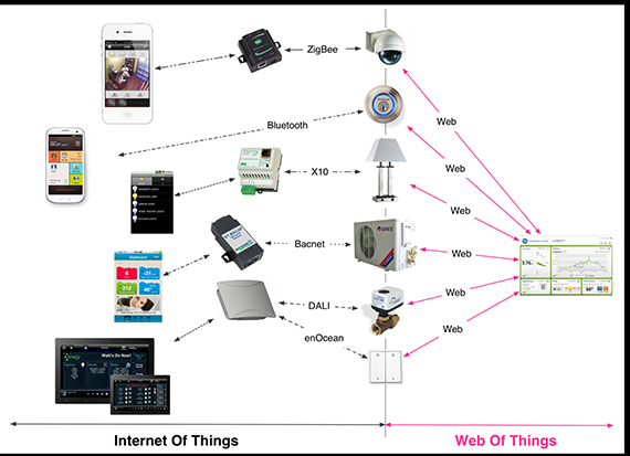 Image courtesy of Dominique Guinard and EVRYTHNG.[/caption]
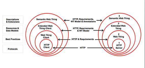 Image courtesy of Dominique Guinard and EVRYTHNG.[/caption]
 Image courtesy of Dominique Guinard and EVRYTHNG.[/caption]


